PivotTables: A Step-by-Step Guide for Beginners

Excel PivotTables Tutorial for Beginners

PivotTables are a powerful tool in spreadsheet programs like Microsoft Excel, designed to summarize, analyze, sort, organize, and present large sets of data in a format that makes it easier to understand and analyze. They allow users to group and pivot data dynamically, showing summaries, averages, counts, or other statistical measures in a table format. allowing users to extract significant patterns, trends, and insights from data by enabling them to group and rearrange information, calculate summaries and aggregates, and compare various data points with ease.

The significance of PivotTables in data analysis lies in their ability to handle and process large datasets without requiring complex formulas or programming. Users can quickly generate reports, perform exploratory data analysis, and make data-driven decisions by simply dragging and dropping fields into different parts of the table.

---

Key features and benefits include:

• Data Summarization: PivotTables can automatically calculate sums, averages, counts, and other aggregates, making it easy to understand large datasets.
• Flexibility: They allow for quick reorganization of data, enabling users to view information from different perspectives and discover hidden patterns.
• Interactive Exploration: You can drill down into details or roll up to see summaries, offering a detailed and high-level overview.
• Filtering and Sorting: PivotTables provide options to filter and sort data, focusing on specific segments that are of interest.
• Time-saving: Save your time and effort, to analyze complex datasets.

In summary, PivotTables are essential features for anyone involved in data analysis, offering a user-friendly and powerful way to explore and interpret data.

---

What are PivotTables?

1. Summarization: PivotTables can quickly aggregate large amounts of data to provide a summary view. (example, summing sales figures across different regions or time periods without writing complex formulas.)
2. Analysis: They facilitate deep data analysis by allowing users to drag and drop fields to different axes of the table, instantly reorganizing the information to highlight different aspects.
3. Exploration: PivotTables make it easy to explore and interrogate data. Users can drill down into summary data to view detailed source records, helping to uncover the underlying causes behind the trends.
4. Presentation: With PivotTables, presenting data in a clear and concise way is straightforward. They can be quickly formatted to highlight key information, making them invaluable for reports and decision-making processes.

Benefits of Using PivotTables for Data Analysis

1. Simplification of Large Data Sets: PivotTables can turn extensive, complicated data sets into clear summaries, making it easier to understand and analyze vast amounts of information.
2. Easy Identification of Trends and Patterns: By reorganizing data, PivotTables help users spot trends, patterns, and anomalies. This can be crucial for forecasting, strategizing, and making informed decisions.
3. Dynamic Data Interactions: PivotTables are interactive, allowing users to change the structure of the data dynamically. This interactivity aids in examining different scenarios or answering specific business questions on the fly.
4. No Formulas Required: To summarize data in PivotTables, users don’t need to write complex formulas. This makes them accessible to beginners and reduces the risk of errors in data calculation.
5. Efficient Data Comparison: PivotTables enable the comparison of data points from different perspectives. (example, comparing sales performance across different time periods or geographical locations is straightforward.)

Preparing Your Data for a PivotTable

Creating a PivotTable in Excel begins with organizing your data properly. Here are concise guidelines to ensure your data is ready for PivotTable analysis:

1. Ensure Data is in Tabular Format:
   • Arrange your data in rows and columns, with each row containing a record and each column a different variable (e.g., sales, dates, regions)
2. No Blank Rows or Columns:
   • Eliminate any blank rows and columns in your dataset. These can disrupt the PivotTable’s ability to accurately analyze your data.
3. Clear Headers for Each Column:
   • Each column should have a unique, descriptive header. This not only clarifies the data but also assists in creating more understandable PivotTables.
4. Remove Duplicate Entries:
   • Duplicate data can skew your analysis. Ensure each record is unique to maintain the integrity of your insights.
5. Consistent Data within Columns:
   • Ensure that each piece of data in a column is consistent in type (e.g., all text, dates, or numbers). Mixing types can lead to errors in analysis.
6. Use a Single Table:
   • If possible, consolidate your data into one table. This simplification streamlines the creation of a PivotTable.

By following these guidelines, you’ll have a solid foundation for creating PivotTables that can efficiently analyze and bring insights to your data, making complex datasets manageable and understandable.

---

Creating Your First PivotTable

Follow these steps to create a PivotTable in Excel, a powerful tool for summarizing and analyzing data sets.

Selecting Your Data:

• Open your dataset in Excel. Ensure your data meets the preparation criteria (e.g., no blank rows/columns, tabular format, clear headers).
• Highlight the data range you want to include in your PivotTable. If your data is well-organized and each column has a clear header, you can simply click any single cell within your dataset without highlighting everything.

Inserting a PivotTable:

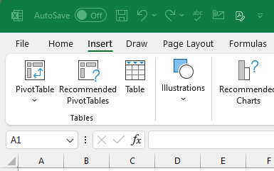
1. Navigate to the Insert tab on the Excel ribbon.
2. Click on the PivotTable button. A dialog box will appear.
3. Choose where to place your PivotTable:
   • New Worksheet: Ideal for most cases, as it keeps the PivotTable separate from your data.
   • Existing Worksheet: Choose this option if you want the PivotTable close to your original data. Specify the location by selecting a cell in the ‘Location’ field.

Adding Fields to Your PivotTable

1. Understand the PivotTable Field List: This appears on the right side of Excel after inserting your PivotTable. It lists all column headers from your selected data.
2. Drag fields into the Rows, Columns, Values, and Filters areas:
   • Rows and Columns: Decide how to categorize your data. Dragging a field to ‘Rows’ or ‘Columns’ organizes your data accordingly.
   • Values: Typically numerical data you want to analyze, like sales numbers. Excel will automatically calculate totals, averages, or counts based on these values.
   • Filters: Fields placed here allow you to filter the entire PivotTable based on the selected criteria.

Exploring Your Data

• Rearrange fields by dragging them between Rows, Columns, Values, and Filters to discover different insights. This flexibility is a key strength of PivotTables.
• Use filters to narrow down your data for more specific analysis. Filters can be applied both from the Filters area and directly from labels in Rows and Columns.
• Experiment with Value Field Settings by right-clicking on a value in your PivotTable and selecting “Value Field Settings” to change how your data is summarized (sum, average, count, etc.).

By following these steps, you can begin to uncover trends, patterns, and insights in your data that were not immediately evident, demonstrating the power of Pivot

---

Customizing Your PivotTable

Customizing and formatting your PivotTable enhances readability and tailors the analysis to your needs. Here’s how to do it:

1. Change the Summary Function:
   • Right-click a value in the PivotTable, select “Value Field Settings,” and choose a different calculation method (e.g., Sum, Count, Average).
2. Apply Styles:
   • Go to the PivotTable Design tab to select from various predefined styles to quickly change the appearance of your PivotTable.
3. Adjust Field Settings:
   • Fine-tune how data is displayed by right-clicking a field in the Rows or Columns area and exploring options like “Field Settings” for layout adjustments.
4. Group Data:
   • Right-click on a data point in Rows or Columns, then select “Group.” This feature is useful for detailed analysis, allowing you to group dates, numbers, or items for a consolidated view.

By leveraging these customization options, you can make your PivotTable more insightful and aligned with your analytical goals.

Refreshing Your PivotTable

How to Refresh:

• Right-click inside your PivotTable and select “Refresh” to update it with any changes from your data source.

Automatic Refresh Options:

• Go to PivotTable Options > Data tab, and enable “Refresh data when opening the file” for automatic updates.

Best Practices for Using PivotTables

• Use Dynamic Data Ranges: Convert your data range into an Excel Table. This ensures your PivotTable automatically includes new data as you add it.
• Avoid Manual Edits: Don’t directly edit the data in a PivotTable. Instead, make changes to the source data and refresh the PivotTable.
• Regularly Refresh: Keep your data accurate by frequently refreshing your PivotTable, especially after modifying the source data.

---

Common Pitfalls and How to Avoid Them

• Data Not Updating: Ensure your data source range includes all relevant data, especially if not using an Excel Table. Refresh after changes.
• Incorrect Summary Calculations: Double-check that your “Values” field settings match the intended analysis (Sum, Count, Average, etc.).

---

Conclusion

PivotTables transform complex data analysis, making it accessible and manageable for beginners. Dive into creating PivotTables with your datasets to uncover insights and improve decision-making.

Resources

• Microsoft Office Support
• ExcelJet
• Excel Shortcut Keys

FAQ Section

• Q: Why doesn’t my PivotTable reflect the latest data?
  • A: Ensure you refresh your PivotTable after any changes to the source data.
• Q: How can I make my PivotTable automatically include new data?
  • A: Convert your data range into an Excel Table before creating your PivotTable.
• Q: Can I change the summary function in my PivotTable?
  • A: Yes, right-click a value, select “Value Field Settings,” and choose the desired summary function.

Practicing with PivotTables and exploring their features will help you become proficient in data analysis, turning seemingly complex information into actionable insights.